import numpy as np
from scipy.stats import binom
import pandas as pd
from scipy.stats import norm
from statsmodels.formula.api import ols
import matplotlib.pyplot as plt第5章のPythonコード
第5章 推測統計の基礎
モジュールのインポート
5.1 統計的仮説検定の考え方
5.1.3 コイン投げの例
p40 = binom.cdf(k = 40, n = 100, p = 0.5)
p60 = binom.cdf(k = 60, n = 100, p = 0.5)

print(p60 - p40)0.95395593307065735.2 平均値の検定
5.2.5 Rによる例題演習
simdata = pd.read_csv('distributions.csv')

sample_mean = simdata.mean(numeric_only = True)[0]
sample_var = simdata.var(numeric_only = True)[0]

print(
    "Mean of A: ", sample_mean, "\n",
    "Varicane of A: ", sample_var, "\n",
    "t-value: ", (100 ** 0.5) * (sample_var ** -0.5) * (sample_mean)
)
Mean of A: 2.0423230835000004
Varicane of A: 0.37278460765476673
t-value: 33.449949007060785.2.6 \(p\)値
1 - norm.cdf(x = 1.250113) + norm.cdf(x = -1.250113)0.211258271555670785.3 回帰係数の検定
5.3.2 \(\hat{\beta}_1\)の分布のシミュレーション
np.random.seed(2022)

X = np.random.normal(loc = 0, scale = 1, size = 1000)
Y = 1 + 5 * X + np.random.normal(loc = 0, scale = 1, size = 1000)

mydata = pd.DataFrame(np.array([X, Y]).transpose(), columns = ['X', 'Y'])

beta1 = ols('Y ~ X', data = mydata).fit().params[1]
S = 10000
beta1 = np.zeros(S) # 結果の保存
for i in range(S): # 繰り返し開始
X = np.random.normal(loc = 0, scale = 1, size = 1000)
Y = 1 + 5 * X + np.random.normal(loc = 0, scale = 1, size = 1000)
mydata = pd.DataFrame(np.array([X, Y]).transpose(), columns = ['X', 'Y'])
beta1[i] = ols('Y ~ X', data = mydata).fit().params[1]
# 繰り返し終了pd.DataFrame(beta1).describe()| 0 | |
|---|---|
| count | 10000.000000 |
| mean | 5.000060 |
| std | 0.031486 |
| min | 4.887715 |
| 25% | 4.978288 |
| 50% | 4.999855 |
| 75% | 5.021525 |
| max | 5.120464 |
plt.hist(beta1, bins = 20)
plt.show()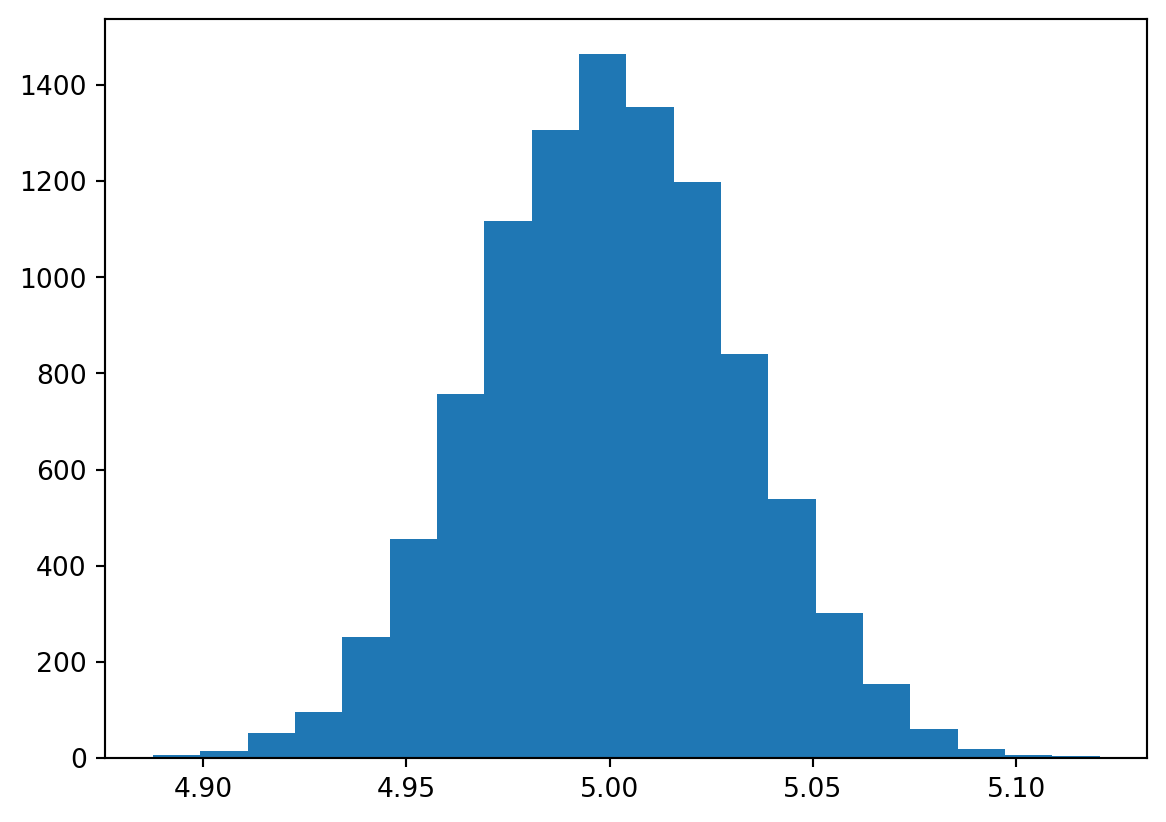
5.3.6 Rによる分析例
wagedata = pd.read_csv('wage.csv')

wagedata['log_wage'] = np.log(wagedata['wage'])

result = ols('log_wage ~ educ + exper', data = wagedata).fit()
print(result.summary())
OLS Regression Results
==============================================================================
Dep. Variable: log_wage R-squared: 0.181
Model: OLS Adj. R-squared: 0.181
Method: Least Squares F-statistic: 333.0
Date: Wed, 05 Jun 2024 Prob (F-statistic): 2.32e-131
Time: 18:21:20 Log-Likelihood: -1524.1
No. Observations: 3010 AIC: 3054.
Df Residuals: 3007 BIC: 3072.
Df Model: 2
Covariance Type: nonrobust
==============================================================================
coef std err t P>|t| [0.025 0.975]
------------------------------------------------------------------------------
Intercept 4.6660 0.064 73.147 0.000 4.541 4.791
educ 0.0932 0.004 25.796 0.000 0.086 0.100
exper 0.0407 0.002 17.417 0.000 0.036 0.045
==============================================================================
Omnibus: 37.191 Durbin-Watson: 1.739
Prob(Omnibus): 0.000 Jarque-Bera (JB): 41.243
Skew: -0.228 Prob(JB): 1.11e-09
Kurtosis: 3.348 Cond. No. 140.
==============================================================================
Notes:
[1] Standard Errors assume that the covariance matrix of the errors is correctly specified.print(0.0932 / 0.004)23.35.4 信頼区間
5.4.2 Rによる分析例
result = ols('log_wage ~ educ + exper', data = wagedata).fit()

print(result.summary())
OLS Regression Results
==============================================================================
Dep. Variable: log_wage R-squared: 0.181
Model: OLS Adj. R-squared: 0.181
Method: Least Squares F-statistic: 333.0
Date: Wed, 05 Jun 2024 Prob (F-statistic): 2.32e-131
Time: 18:21:20 Log-Likelihood: -1524.1
No. Observations: 3010 AIC: 3054.
Df Residuals: 3007 BIC: 3072.
Df Model: 2
Covariance Type: nonrobust
==============================================================================
coef std err t P>|t| [0.025 0.975]
------------------------------------------------------------------------------
Intercept 4.6660 0.064 73.147 0.000 4.541 4.791
educ 0.0932 0.004 25.796 0.000 0.086 0.100
exper 0.0407 0.002 17.417 0.000 0.036 0.045
==============================================================================
Omnibus: 37.191 Durbin-Watson: 1.739
Prob(Omnibus): 0.000 Jarque-Bera (JB): 41.243
Skew: -0.228 Prob(JB): 1.11e-09
Kurtosis: 3.348 Cond. No. 140.
==============================================================================
Notes:
[1] Standard Errors assume that the covariance matrix of the errors is correctly specified.betahat = result.params
sigma = result.bse
lower = betahat - 1.96 * sigma
upper = betahat + 1.96 * sigma
pd.concat([lower, upper], axis = 1)| 0 | 1 | |
|---|---|---|
| Intercept | 4.541006 | 4.791063 |
| educ | 0.086089 | 0.100247 |
| exper | 0.036082 | 0.045233 |
result.conf_int(alpha = 0.05)| 0 | 1 | |
|---|---|---|
| Intercept | 4.540958 | 4.791111 |
| educ | 0.086086 | 0.100250 |
| exper | 0.036080 | 0.045235 |
result.conf_int(alpha = 0.01)| 0 | 1 | |
|---|---|---|
| Intercept | 4.501618 | 4.830451 |
| educ | 0.083859 | 0.102477 |
| exper | 0.034641 | 0.046674 |